Previziuni cuibărite: Analizarea relației dintre dolarul și tendințele pieței bursiere

Opinia predominantă este că, deoarece țările exportă mai multe bunuri în SUA decât le exportă, rezultând un deficit comercial. În schimbul exporturilor lor, aceste țări primesc dolari americani, pe care le folosesc adesea pentru a achiziționa obligațiuni și stocuri guvernamentale americane. În timp, acest proces contribuie la consolidarea dolarului.

Cu toate acestea, graficul de mai jos indică o corelație negativă între piața bursieră și indicele dolarului în perioadele recente.

Cod sursă:

library(tidyverse)
library(tidymodels)
library(timetk)
library(modeltime)
library(tidyquant)
library(splines)
library(ggh4x)

#US Dollar Index (DX-Y.NYB) 
df_dollar_index <- 
  tq_get("DX-Y.NYB", to = "2025-07-01") %>% 
  tq_transmute(select = close,
               mutate_fun = to.monthly,
               col_rename = "value") %>% 
  mutate(date = as.Date(date),
         id = "Dollar Index")

#S&P 500
df_sp500 <- 
  tq_get("^GSPC", to = "2025-07-01") %>% 
  tq_transmute(select = close,
               mutate_fun = to.monthly,
               col_rename = "value") %>% 
  mutate(date = as.Date(date),
         id = "S&P 500")

#Panel Data
df_panel <- 
  df_dollar_index %>% 
  bind_rows(df_sp500) %>% 
  mutate(id = as_factor(id))


df_panel %>%
  group_by(id) %>%
  plot_time_series(
    date, value, .interactive = F, .facet_ncol = 1
  ) +
  scale_y_continuous(labels = scales::label_currency())

#Nested data
nested_data_tbl <- 
  df_panel %>%
  
  # 1. Extending: We'll predict 52 weeks into the future.
  extend_timeseries(
    .id_var        = id,
    .date_var      = date,
    .length_future = 12
  ) %>%
  
  # 2. Nesting: We'll group by id, and create a future dataset
  #    that forecasts 52 weeks of extended data and
  #    an actual dataset that contains 104 weeks (2-years of data)
  nest_timeseries(
    .id_var        = id,
    .length_future = 12,
    .length_actual = 12*2
  ) %>%
  
  # 3. Splitting: We'll take the actual data and create splits
  #    for accuracy and confidence interval estimation of 52 weeks (test)
  #    and the rest is training data
  split_nested_timeseries(
    .length_test = 12
  )


#Nested Modeltime Workflow
#Create Tidymodels Workflows

#Prophet
rec_prophet <- 
  recipe(value ~ date, extract_nested_train_split(nested_data_tbl))

wflw_prophet <- 
  workflow() %>%
  add_model(
    prophet_reg("regression") %>% 
      set_engine("prophet")
  ) %>%
  add_recipe(rec_prophet)


#Linear Regression
rec_glmnet <- 
  recipe(value ~ date, data = extract_nested_train_split(nested_data_tbl)) %>% 
  step_mutate(date_num = as.numeric(date)) %>% 
  step_date(date, features = "month") %>% 
  step_ns(date_num) %>% 
  step_rm(date) %>% 
  step_dummy(all_nominal_predictors(), one_hot = TRUE) %>% 
  step_normalize(all_numeric_predictors()) 

wflw_glmnet <- 
  workflow() %>%
  add_model(linear_reg(penalty = 0.2) %>%
              set_engine("glmnet")) %>%
  add_recipe(rec_glmnet)

#XGBoost
rec_xgb <- 
  recipe(value ~ date, extract_nested_train_split(nested_data_tbl)) %>%
  step_timeseries_signature(date) %>%
  step_rm(date) %>%
  step_zv(all_predictors()) %>%
  step_dummy(all_nominal_predictors(), one_hot = TRUE)

wflw_xgb <- 
  workflow() %>%
  add_model(boost_tree("regression") %>% set_engine("xgboost")) %>%
  add_recipe(rec_xgb)

#Nested Modeltime Tables
nested_modeltime_tbl <- 
  modeltime_nested_fit(
  # Nested data 
  nested_data = nested_data_tbl,
  
  # Add workflows
  wflw_prophet,
  wflw_glmnet,
  wflw_xgb
)

#Extract Nested Test Accuracy
best_nested_modeltime_tbl <- 
  nested_modeltime_tbl %>%
  modeltime_nested_select_best(
    metric                = "mape", 
    minimize              = TRUE, 
    filter_test_forecasts = TRUE
  )

#Extract Nested Best Model Report
best_nested_modeltime_tbl %>%
  extract_nested_best_model_report()

#Extract Nested Test Accuracy
nested_modeltime_tbl %>% 
  extract_nested_test_accuracy() %>%
  table_modeltime_accuracy()


#Extract Nested Best Test Forecasts
best_nested_modeltime_tbl %>%
  extract_nested_test_forecast() %>%
  group_by(id) %>%
  plot_modeltime_forecast(
    .facet_ncol  = 1,
    .interactive = FALSE,
    .line_size = 1
  ) +
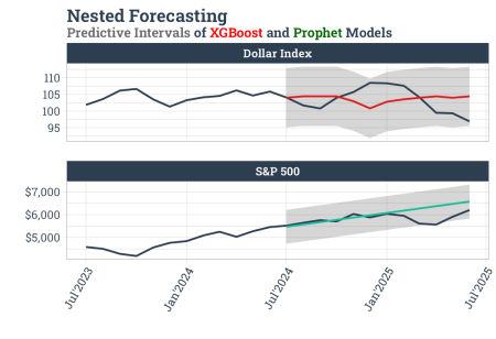
  labs(title = "Nested Forecasting", 
       subtitle = "Predictive Intervals of XGBoost and Prophet Models", 
       y = "", x = "") + 
  facet_wrap(~ id, 
             ncol = 1, 
             scales = "free_y") + 
  facetted_pos_scales(
    y = list(
      id == "Dollar Index" ~ scale_y_continuous(labels = scales::number_format()),
      id == "S&P 500" ~ scale_y_continuous(labels = scales::label_currency())
    )
  ) +
  scale_x_date(labels = scales::label_date("%b'%Y")) +
  theme_tq(base_family = "Roboto Slab", base_size = 16) +
  theme(plot.subtitle = ggtext::element_markdown(face = "bold"),
        plot.title = element_text(face = "bold"),
        strip.text = element_text(face = "bold"),
        axis.text.x = element_text(angle = 60, hjust = 1, vjust = 1),
        legend.position = "none")