Previziuni cuibărite cu scânteie: tendințe blockchain ETF

Bitcoin a atins un nivel maxim de 125.664 dolari la 5 octombrie. Această creștere a fost alimentată de un flux net istoric de 3,24 miliarde de dolari în ETF-uri Bitcoin Spot și în creștere a cererii publice.

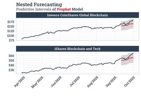
În acest articol, vom prezice tendința a două ETF -uri blockchain folosind prognoză cuibărită cu backend -ul scânteie.

Nu am putut folosi valorile întârziate și netezind în rețete, deoarece N / A a provocat o problemă în structura datelor cuibărite.

library(modeltime)
library(timetk)
library(tidymodels)
library(dplyr)
library(tidyquant)
library(sparklyr)

#Connection
sc <- spark_connect(master = "local")

#Setup the Spark Backend
parallel_start(sc, .method = "spark")

#Invesco CoinShares Global Blockchain UCITS ETF (BCHN.L)
df_bchn <- 
  tq_get("BCHN.L") %>% 
  select(date, 'Invesco CoinShares Global Blockchain' = close) 

#iShares Blockchain and Tech ETF (IBLC)
df_iblc <- 
  tq_get("IBLC") %>% 
  select(date, 'iShares Blockchain and Tech' = close) 

#Creating the survey data
df_survey <- 
  df_bchn %>% 
  left_join(df_iblc) %>% 
  pivot_longer(-date,
               names_to = "id",
               values_to = "value") %>% 
  filter(date >= last(date) - months(6)) %>% 
  drop_na()


#Nested Data
nested_data_tbl <- 
  df_survey %>%
  dplyr::select(id, 
                date = date, 
                value = value) %>%
  extend_timeseries(
    .id_var        = id,
    .date_var      = date,
    .length_future = 15
  ) %>%
  nest_timeseries(
    .id_var        = id,
    .length_future = 15
  ) %>%
  
  split_nested_timeseries(
    .length_test = 15
  )


#Modeling
  
#XGBoost
rec_xgb <- 
  recipe(value ~ ., extract_nested_train_split(nested_data_tbl)) %>%
  step_timeseries_signature(date) %>%
  step_rm(date) %>%
  step_dummy(all_nominal_predictors(), one_hot = TRUE) %>% 
  step_zv(all_predictors()) %>%
  step_impute_linear(all_numeric_predictors())

wflw_xgb <- 
  workflow() %>%
  add_model(boost_tree("regression") %>% 
            set_engine("xgboost")) %>%
  add_recipe(rec_xgb)


#Prophet
rec_prophet <- 
  recipe(value ~ date, extract_nested_train_split(nested_data_tbl)) %>% 
  step_date(date, features = c("dow", "month", "year", "doy")) %>% 
  step_dummy(all_nominal_predictors(), one_hot = TRUE) %>% 
  step_zv(all_predictors()) %>%
  step_impute_linear(all_numeric_predictors())

wflw_prophet <- 
  workflow() %>%
  add_model(
    prophet_reg("regression") %>% 
      set_engine("prophet",
                 seasonality_yearly = FALSE,
                 seasonality_weekly = TRUE,
                 seasonality_daily = TRUE)) %>%
  add_recipe(rec_prophet)


#Nested Forecasting with Spark
nested_modeltime_tbl <- 
  nested_data_tbl %>%
  modeltime_nested_fit(
    wflw_xgb,
    wflw_prophet,
    control = control_nested_fit(allow_par = TRUE, verbose = TRUE)
  )

#Model Test Accuracy
nested_modeltime_tbl %>%
  extract_nested_test_accuracy() %>%
  table_modeltime_accuracy(.interactive = T)


#Extract Nested Test Accuracy
best_nested_modeltime_tbl <- 
  nested_modeltime_tbl %>%
  modeltime_nested_select_best(
    metric                = "mape", 
    minimize              = TRUE, 
    filter_test_forecasts = TRUE
  )

#Extract Nested Best Model Report
best_nested_modeltime_tbl %>%
  extract_nested_best_model_report()


#Extract Nested Best Test Forecasts
best_nested_modeltime_tbl %>%
  extract_nested_test_forecast() %>%
  group_by(id) %>%
  plot_modeltime_forecast(
    .facet_ncol  = 1,
    .interactive = FALSE,
    .line_size = 1
  ) +
  labs(title = "Nested Forecasting", 
       subtitle = "Predictive Intervals of Prophet Model", 
       y = "", x = "") + 
  facet_wrap(~ id, 
             ncol = 1, 
             scales = "free_y") + 
  scale_y_continuous(labels = scales::label_currency()) +
  scale_x_date(labels = scales::label_date("%b'%Y"),
               date_breaks = "30 days") +
  theme_tq(base_family = "Roboto Slab", base_size = 16) +
  theme(plot.subtitle = ggtext::element_markdown(face = "bold"),
        plot.title = element_text(face = "bold"),
        strip.text = element_text(face = "bold"),
        axis.text = element_text(face = "bold"),
        axis.text.x = element_text(angle = 45, hjust = 1, vjust = 1),
        legend.position = "none")