Această postare este a treia parte a https://thierrymoudiki.github.io/blog/2025/12/07/r/forecasting/ARIMA-Pricing și https://thierrymoudiki.github.io/blog/2026/02/01/r/Semi-parametric-MarketPriceofRisk-The. Aceste postări au arătat cum să utilizați ARIMA și Theta ca preț de piață al riscului, pentru a stabili apoi opțiunile în conformitate cu o măsură neutră din punct de vedere al riscului prin reeșantionare martingale inovații.
După ce m-am gândit mai mult la asta, iată o versiune condensată a postărilor anterioare, cu câteva formule și exemple bogate de cod R.
1. Stabilirea pieței
Lasă
- (S_t) = prețul activului
- (r) = rata fără risc
- (T) = maturitate
Definiți proces de preț redus
(D_t = e^{-rt} S_t)
Conform principiului fără arbitraj (teorema fundamentală a prețului activelor), există o măsură de probabilitate (Q) astfel încât
(E_Q(D_t mid mathcal{F}_{t-1}) = D_{t-1})
deci (D_t) este a martingale.
Având în vedere căile de preț simulate sau observate (S_t), calculați
(D_t = e^{-rt} S_t)
Definiți incremente
(Delta D_t = D_t – D_{t-1})
Montați un filtru de serie de timp
(Delta D_t = f(Delta D_{t-1}, ldots, Delta D_{tp}) + varepsilon_t)
unde
(E(varepsilon_t) = 0)
3. Distribuția inovației Bootstrap
Lasă
({varepsilon_1, ldots, varepsilon_T})
fie inovaţiile empirice.
Generați reeșantioane bootstrap
(varepsilon_t^{(i)}, quad i = 1, ldots, N)
folosind bootstrap staționar. Aceste secvențe definesc legea inovării.
4. Reconstrucție Martingale
Definiți recursiv procesul actualizat:
(D_0 = S_0) (D_t = D_{t-1} + varepsilon_t)
ceea ce presupune
(D_t = S_0 + sum_{i=1}^{t} varepsilon_i)
Din moment ce
(E(varepsilon_t) = 0)
obținem
(E(D_t) = E(S_0 + sum_{i=1}^{t} varepsilon_i) = S_0 + sum_{i=1}^{t} E(varepsilon_i) = S_0)
5. Proces de preț neutru față de risc
Recuperați procesul de preț
(S_t = e^{rt} D_t)
Apoi
(E(e^{-rt} S_t) = S_0)
care satisface stare de risc neutru.
6. Prețuri Monte Carlo
Pentru payoff (H(S_T)), prețul derivatului este
(V_0 = e^{-rT} E_Q(H(S_T)))
Estimată de Monte Carlo:
(V_0 aprox e^{-rT} frac{1}{N} sum_{i=1}^{N} H(S_T^{(i)}))
Exemplu (apel european):
(C_0 = e^{-rT} E_Q(max(S_T – K, 0)))
Iată codul R pentru întregul proces:
library(esgtoolkit)
library(forecast)
set.seed(123)
n <- 250L
h <- 5
freq <- "daily"
r <- 0.05
maturity <- 5
S0 <- 100
mu <- 0.08
sigma <- 0.04
n_sims <- 5000L
# Simulate under physical measure with stochastic volatility and jumps
sim_GBM <- esgtoolkit::simdiff(
n = n,
horizon = h,
frequency = freq,
x0 = S0,
theta1 = mu,
theta2 = sigma
)
sim_SVJD <- esgtoolkit::rsvjd(n = n, r0 = mu)
sim_Heston <- esgtoolkit::rsvjd(
n = n,
r0 = mu,
lambda = 0,
mu_J = 0,
sigma_J = 0
)
# This exp(-r*t)*S_t
discounted_prices_GBM <- esgtoolkit::esgdiscountfactor(r = r, X = sim_GBM)
discounted_prices_SVJD <- esgtoolkit::esgdiscountfactor(r = r, X = sim_SVJD)
discounted_prices_Heston <- esgtoolkit::esgdiscountfactor(r = r, X = sim_Heston)
# Take the first difference of exp(-r*t)*S_t
# (we want a center first difference in Q)
diff_martingale_GBM <- diff(discounted_prices_GBM)
diff_martingale_Heston <- diff(discounted_prices_Heston)
diff_martingale_SVJD <- diff(discounted_prices_SVJD)
# Adjust a time series filter the martingale difference
choice_process <- "GBM"
choice_filter <- "auto.arima"
diff_martingale <- switch(choice_process,
GBM = diff_martingale_GBM,
Heston = diff_martingale_Heston,
SVJD = diff_martingale_SVJD)
n_dates <- nrow(diff_martingale)
n_dates_1 <- n_dates - 1
resids_matrix <- matrix(0, nrow = n_dates_1, ncol = n)
pb <- utils::txtProgressBar(min = 0, max = n, style = 3L)
if (choice_filter == "AR(1)")
{
for (j in 1:n)
{
y <- diff_martingale(-1, j)
X <- matrix(diff_martingale(seq_len(n_dates_1), j), ncol = 1)
fit_lm <- .lm.fit(x = X, y = y)
fitted_values <- X %*% fit_lm$coef
resids_matrix(, j) <- y - fitted_values
utils::setTxtProgressBar(pb, j)
}
close(pb)
}
if (choice_filter == "auto.arima"){
for (j in 1:n)
{
y <- diff_martingale(-1, j)
resids_matrix(, j) <- residuals(auto.arima(y, allowmean = FALSE))
utils::setTxtProgressBar(pb, j)
}
close(pb)
}
pvals <- sapply(1:n, function(j)
Box.test(resids_matrix(, j), type = "Ljung-Box")$p.value)
# Keep only stationary residuals (non-reject null at 5% level)
stationary_cols <- which(pvals > 0.05)
resids_stationary <- resids_matrix(, stationary_cols)
print(dim(resids_stationary))
centered_resids_stationary <- scale(resids_stationary, center = TRUE, scale = FALSE)(, )
centered_resids_stationary <- ts(centered_resids_stationary,
end = end(sim_GBM),
frequency = frequency(sim_GBM))
# resample_centered_resids has nrow = number of dates, ncol = n_sims
resampled_centered_resids <- list()
n_resids_stationary <- dim(resids_stationary)(2)
n_times <- ceiling(n_sims/n_resids_stationary)
pb <- utils::txtProgressBar(min = 0, max = n_times, style = 3L)
for (i in seq_len(n_times))
{
set.seed(123 + i*100)
resampled_centered_resids((i)) <- apply(centered_resids_stationary, 2,
function(x) tseries::tsbootstrap(x, nb=1,
type="stationary"))
utils::setTxtProgressBar(pb, i)
}
close(pb)
resampled_centered_resids_matrix <- do.call(cbind, resampled_centered_resids)(, seq_len(n_sims))
# Convert to ts object with proper time attributes
resampled_ts <- ts(resampled_centered_resids_matrix,
start = start(centered_resids_stationary),
end = end(centered_resids_stationary),
frequency = frequency(centered_resids_stationary))
# Check dimensions: should be (n_dates-1) x n_sims
print(dim(resampled_ts))
# At time t = 0, diff_martingale process is equal is D_0 = S_0 (exp(-r * 0)*S_0)
# First cumsum the process to get exp(-r*t)*S_t
# Then multiply by exp(r*t) to have a process in risk neutral probability
# Step 1: Start with S0 at t=0
D0 <- S0 # since exp(-r*0) = 1
# Step 2: Cumsum to get discounted prices (e^{-rt} * S_t) under Q
# Add D0 as first row, then cumsum of innovations
discounted_paths <- D0 + apply(resampled_ts, 2, cumsum) # t=1..T
discounted_paths <- rbind(D0, discounted_paths)
discounted_paths <- ts(as.matrix(discounted_paths), start=start(sim_GBM),
frequency = frequency(sim_GBM))
time_points <- time(discounted_paths)
risk_neutral_prices <- ts(discounted_paths * exp(r * time_points),
start=start(sim_GBM),
frequency = frequency(sim_GBM))
head(risk_neutral_prices(, 1:5))
esgplotbands(risk_neutral_prices)
# =============================================================================
# I. Basic diagnostics
# =============================================================================
# No negative prices (log-normal support check)
n_negative <- sum(risk_neutral_prices < 0, na.rm = TRUE)
cat("Negative prices:", n_negative, "n")
stopifnot(n_negative == 0)
# Terminal distribution summary
S_T <- as.numeric(risk_neutral_prices(nrow(risk_neutral_prices), ))
cat("n--- Terminal price S_T summary ---n")
print(summary(S_T))
cat("Std dev:", sd(S_T), "n")
cat("Skewness:", moments::skewness(S_T), "n")
cat("Excess kurtosis:", moments::kurtosis(S_T) - 3, "n")
# =============================================================================
# II. Martingale checks
# =============================================================================
# E(exp(-r*T) * S_T) should equal S_0
T_years <- h
discount_T <- exp(-r * T_years)
mc_price <- discount_T * mean(S_T)
cat("n--- Martingale check ---n")
cat("S_0 :", S0, "n")
cat("E(exp(-rT) * S_T) :", round(mc_price, 4), "n")
cat("Absolute error :", round(abs(mc_price - S0), 4), "n")
# Check at every time point: mean discounted path should stay ~S0
discounted_paths_check <- risk_neutral_prices * exp(-r * time(risk_neutral_prices))
mean_discounted <- rowMeans(discounted_paths_check)
cat("nMean discounted price (first 6 and last 6 time points):n")
print(round(head(mean_discounted), 4))
print(round(tail(mean_discounted), 4))
# t-test: is E(exp(-rT)*S_T) = S0?
ttest <- t.test(discount_T * S_T-S0, mu = 0)
cat("nt-test H0: E(exp(-rT)*S_T) = S0n")
print(ttest)
# =============================================================================
# III. Distributional tests on log-returns
# =============================================================================
log_returns <- diff(log(risk_neutral_prices))
# Normality of cross-sectional log-returns at terminal date
lr_T <- as.numeric(log_returns(nrow(log_returns), ))
cat("n--- Normality tests on terminal log-returns ---n")
print(shapiro.test(sample(lr_T, min(5000L, length(lr_T))))) # Shapiro-Wilk (max n=5000)
print(ks.test(lr_T, "pnorm", mean(lr_T), sd(lr_T))) # KS vs normal
# Mean log-return should be close to (r - 0.5*sigma^2) * dt
dt <- 1 / frequency(risk_neutral_prices)
mean_lr <- mean(lr_T)
theoretical <- (r - 0.5 * sigma^2) * dt
cat("nMean terminal log-return :", round(mean_lr, 6), "n")
cat("Theoretical (r-s²/2)*dt :", round(theoretical, 6), "n")
# Variance ratio: empirical vs GBM theoretical
# Under GBM: Var(log S_T) = sigma^2 * T
empirical_var <- var(log(S_T))
theoretical_var <- sigma^2 * T_years
cat("n--- Variance ratio check ---n")
cat("Var(log S_T) empirical :", round(empirical_var, 4), "n")
cat("Var(log S_T) GBM theory :", round(theoretical_var, 4), "n")
cat("Ratio :", round(empirical_var / theoretical_var, 4), "n")
# =============================================================================
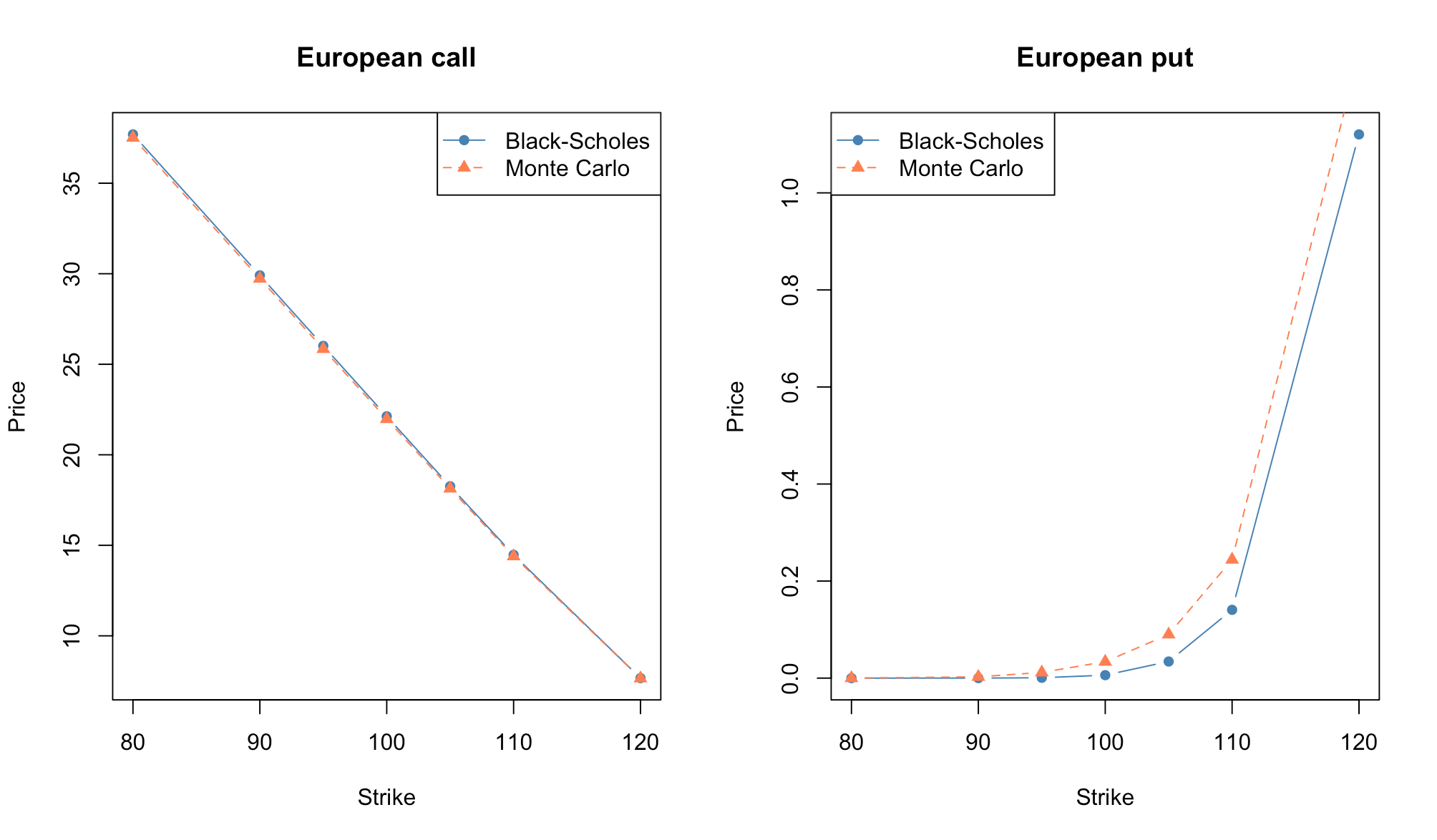
# IV. Option pricing — European calls and puts
# =============================================================================
strikes <- c(80, 90, 95, 100, 105, 110, 120) # ITM to OTM
# -- Monte Carlo prices -------------------------------------------------------
mc_call <- sapply(strikes, function(K)
exp(-r * T_years) * mean(pmax(S_T - K, 0)))
mc_put <- sapply(strikes, function(K)
exp(-r * T_years) * mean(pmax(K - S_T, 0)))
# -- Black-Scholes prices -----------------------------------------------------
bs_call <- function(S, K, r, sigma, T) {
d1 <- (log(S/K) + (r + 0.5*sigma^2)*T) / (sigma*sqrt(T))
d2 <- d1 - sigma*sqrt(T)
S * pnorm(d1) - K * exp(-r*T) * pnorm(d2)
}
bs_put <- function(S, K, r, sigma, T) {
d1 <- (log(S/K) + (r + 0.5*sigma^2)*T) / (sigma*sqrt(T))
d2 <- d1 - sigma*sqrt(T)
K * exp(-r*T) * pnorm(-d2) - S * pnorm(-d1)
}
bsc <- sapply(strikes, function(K) bs_call(S0, K, r, sigma, T_years))
bsp <- sapply(strikes, function(K) bs_put(S0, K, r, sigma, T_years))
# -- Put-call parity check (MC) -----------------------------------------------
# C - P = S0 - K*exp(-rT) (forward parity)
pcp_mc <- mc_call - mc_put
pcp_th <- S0 - strikes * exp(-r * T_years)
pcp_err <- abs(pcp_mc - pcp_th)
# -- Summary table ------------------------------------------------------------
results <- data.frame(
K = strikes,
BS_call = round(bsc, 4),
MC_call = round(mc_call, 4),
err_call = round(abs(mc_call - bsc), 4),
BS_put = round(bsp, 4),
MC_put = round(mc_put, 4),
err_put = round(abs(mc_put - bsp), 4),
PCP_error = round(pcp_err, 4)
)
cat("n--- European option prices: MC vs Black-Scholes ---n")
print(results, row.names = FALSE)
# -- Plot ---------------------------------------------------------------------
par(mfrow = c(1, 2))
plot(strikes, bsc, type = "b", pch = 16, col = "steelblue",
xlab = "Strike", ylab = "Price", main = "European call")
lines(strikes, mc_call, type = "b", pch = 17, col = "coral", lty = 2)
legend("topright", legend = c("Black-Scholes", "Monte Carlo"),
col = c("steelblue", "coral"), pch = c(16, 17), lty = c(1, 2))
plot(strikes, bsp, type = "b", pch = 16, col = "steelblue",
xlab = "Strike", ylab = "Price", main = "European put")
lines(strikes, mc_put, type = "b", pch = 17, col = "coral", lty = 2)
legend("topleft", legend = c("Black-Scholes", "Monte Carlo"),
col = c("steelblue", "coral"), pch = c(16, 17), lty = c(1, 2))
par(mfrow = c(1, 1))