(Acest articol a fost publicat pentru prima dată pe Guillaume Pressiatși cu amabilitate a contribuit la R-bloggeri). (Puteți raporta problema legată de conținutul acestei pagini aici)
Doriți să vă distribuiți conținutul pe R-bloggeri? dați clic aici dacă aveți un blog, sau aici dacă nu aveți.
Această postare minunată de la Jonathan Caroll îmi dă idee să mă joc cu codul ggplot2 și paletele de culori scico:
Vedeți și acest toot de la Stefan Siegert, inspirator!
Am luat codul din toot-ul menționat mai sus, l-am modificat și l-am folosit pentru a mă distra puțin creând grafice care arată ca niște picturi cu imperfecțiuni în jurul marginilor, printre altele.
Una peste alta, cred că este o modalitate bună de a testa paletele de culori.
Când obțineți imagini cu puncte pe inch mai mari, poate fi foarte cool.
# https://mastodon.social/@safest_integer/114296256313964335
library(tidyverse)
crossing(x=0:10, y=x) |>
mutate(dx = rnorm(n(), 0, (y/20)^1.5),
dy = rnorm(n(), 0, (y/20)^1.5)) |>
ggplot() +
geom_tile(aes(x=x+dx, y=y+dy, fill=y), colour="black",
lwd=2, width=1, height=1, alpha=0.8, show.legend=FALSE) +
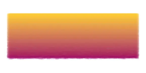
scale_fill_gradient(high="#9f025e", low='#f9c929') +
scale_y_reverse() + theme_void()
library(tidyverse)

crossing(x=8:300, y=x(1:100)) |>
  mutate(dx = rnorm(n(), 0, (y/200)^1.5),
         dy = rnorm(n(), 0, (y/100)^1.5)) |>
  ggplot() +
  geom_tile(aes(x=x+dx, y=y+dy, fill=y), colour=NA,
            lwd=4, width=8, height=4, alpha=0.1,
            show.legend=FALSE) +
  scale_fill_gradient(high="#9f025e", low='#f9c929') +
  scale_y_reverse() + theme_void() +
  coord_fixed()
![]()
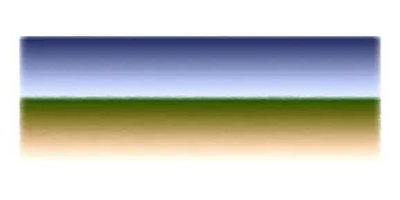
Iată paleta de culori „Oleron” de la scico. Ce paletă frumoasă pentru cei care cunosc această insulă franceză!
library(tidyverse)

crossing(x=8:300, y=x(1:100)) |>
  mutate(dx = rnorm(n(), 0, (y/200)^1.5),
         dy = rnorm(n(), 0, (y/100)^1.5)) |>
  ggplot() +
  geom_tile(aes(x=x+dx, y=y+dy, fill=y), colour=NA,
            lwd=4, width=8, height=4, alpha=0.1,
            show.legend=FALSE) +
  scico::scale_fill_scico(palette = "oleron",
  direction = 1) +
  scale_y_reverse() + theme_void() +
  coord_fixed()
![]()
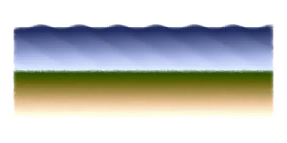
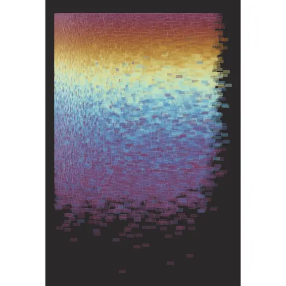
Acum desenând valuri, vedeți în vârful dunei:
crossing(x=8:300, y=x(1:100)) |>
  mutate(dx = rnorm(n(), 0, (y/200)^1.5),
         dy = ifelse(y < 52,
                     rnorm(n(), 0, (y/100)^1.5)+
                       ifelse(x %% 2 == 0,
                              cos(x * 3 + y / 5)*4 +
                                sin(x * 3 + y / 2)*2, 0) / 1.7,
                     rnorm(n(), 0, (y/100)^1.5))) |>
  ggplot() +
  geom_tile(aes(x=x+dx, y=y+dy, fill=y), colour=NA,
            lwd=4, width=8, height=4, alpha=0.2,
            show.legend=FALSE) +
  scico::scale_fill_scico(palette = "oleron", #begin = 0.6,
                          direction = 1) +
  scale_y_reverse() + theme_void() +
  coord_fixed()
Verdele ar putea fi vegetația din dune sau poate alge marine. Albastrul ar putea fi, de asemenea, cerul și vânt, ora albastră, cu siguranță există nisip.
![]()
Înapoi la dreptunghiuri mai mari cu o paletă scico ciclică: romaO.
crossing(x=1:280, y=x) |>
  mutate(dx = rnorm(n(), 0, (x/40)^1.5),
         dy = rnorm(n(), 0, (y/40)^1.5)) |>
  ggplot() +
  geom_tile(aes(x=x+dx, y=y-dy*3, fill=y), colour="white",
            lwd=0.03, width=13, height=6, alpha=0.4,
            show.legend=FALSE) +
  scico::scale_fill_scico(palette = "romaO", #begin = 0.6,
                          direction = 1) +
  scale_y_reverse() + theme_void() +
  theme(panel.background = element_rect(fill = "#2b2828")) +
  coord_fixed()
![]()
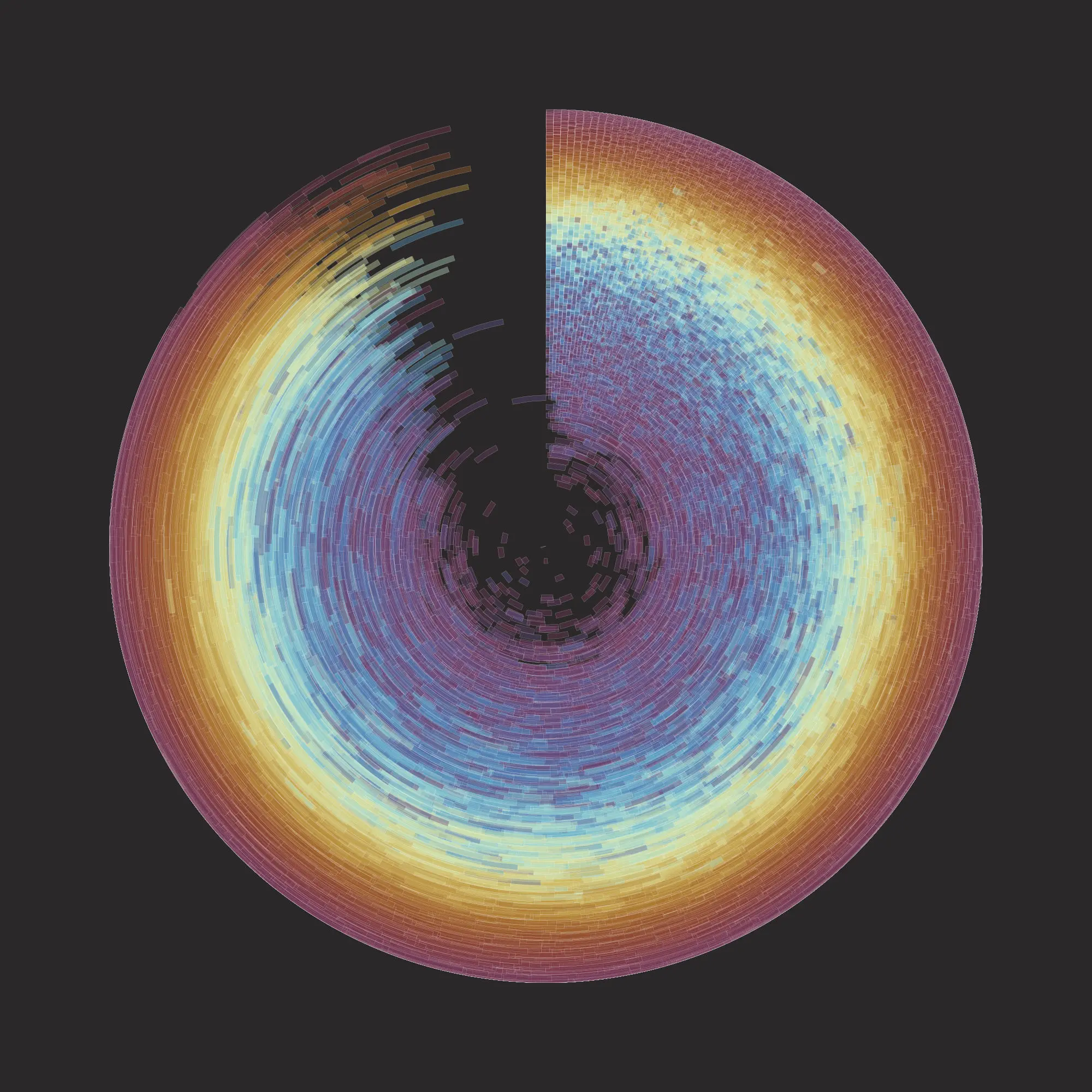
Acum doar joacă-te cu puțin mai multă magie: coord_polar
crossing(x=1:280, y=x) |>
  mutate(dx = rnorm(n(), 0, (x/40)^1.5),
         dy = rnorm(n(), 0, (y/40)^1.5)) |>
  ggplot() +
  geom_tile(aes(x=x+dx, y=y-dy*3, fill=y), colour="white",
            lwd=0.03, width=13, height=6, alpha=0.4,
            show.legend=FALSE) +
  scico::scale_fill_scico(palette = "romaO", #begin = 0.6,
  direction = 1) +
  scale_y_reverse() + theme_void() +
  theme(panel.background = element_rect(fill = "#2b2828")) +
  coord_polar()
![]()
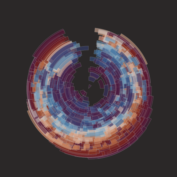
Altul cu vikO paletă:
crossing(x=8:70, y=x(1:30)) |>
  mutate(dx = rnorm(n(), 0, (y/20)^1.5),
         dy = rnorm(n(), 0, (y/10)^1.5)+ ifelse(x %%2 == 0, cos(x * 3 + y / 5)*10, 0)) |>
  ggplot() +
  geom_tile(aes(x=x+dx, y=y+dy, fill=y), colour="grey70",
            lwd=0.1, width=8, height=4, alpha=0.6,
            show.legend=FALSE) +
  scico::scale_fill_scico(palette = "vikO", #begin = 0.6,
                          direction = -1) +
  scale_y_reverse() +
  theme_void() +
  theme(panel.background = element_rect(fill = "#2b2828")) +
  coord_polar(theta = "x")
![]()
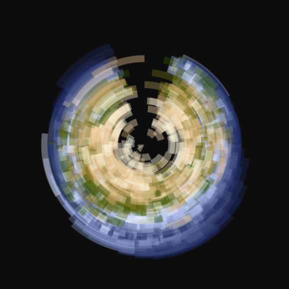
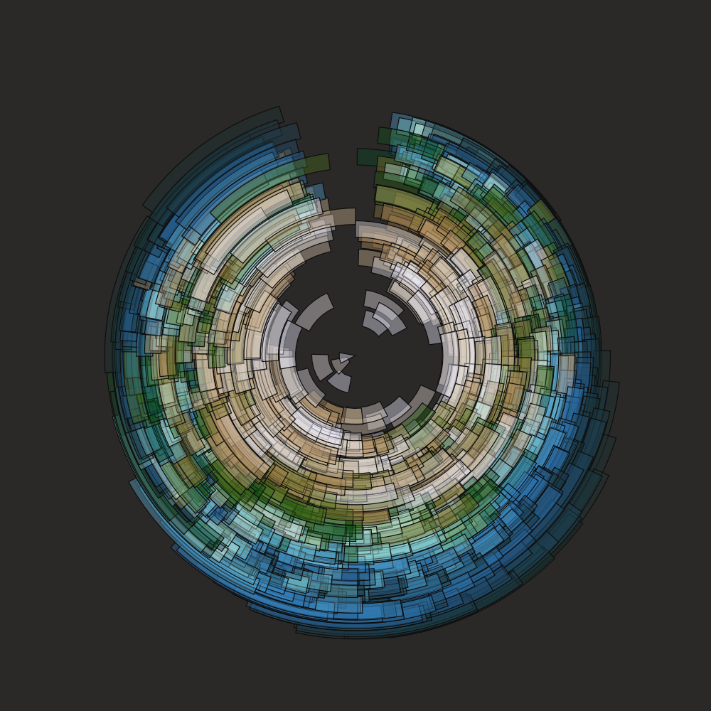
În sfârșit, înapoi la paleta Oleron cu coord_polar:
crossing(x=8:70, y=x(1:30)) |>
  mutate(dx = rnorm(n(), 0, (y/20)^1.5),
         dy = rnorm(n(), 0, (y/10)^1.5)+ ifelse(x %%2 == 0, cos(x * 3 + y / 5)*10, 0)) |>
  ggplot() +
  geom_tile(aes(x=x+dx, y=y+dy, fill=y), colour=NA,
            lwd=1, width=8, height=4, alpha=0.4,
            show.legend=FALSE) +
  scico::scale_fill_scico(palette = "oleron", #begin = 0.6,
                          direction = 1) +
  scale_y_reverse() +
  theme_void() +
  theme(panel.background = element_rect(fill = "grey5")) + ##2b2828
  coord_polar(theta = "x")
Cam ca Pământul, dar nu de pe Lună. Doar de la R.
![]()

bukavu paletă:
crossing(x=8:70, y=x(1:30)) |>
  mutate(dx = rnorm(n(), 0, (y/20)^1.5),
         dy = rnorm(n(), 0, (y/10)^1.5)+ ifelse(x %%2 == 0, cos(x * 3 + y / 5)*10, 0)) |>
  ggplot() +
  geom_tile(aes(x=x+dx, y=y+dy, fill=y), colour="grey5",
            lwd=0.2, width=8, height=4, alpha=0.4,
            show.legend=FALSE) +
  scico::scale_fill_scico(palette = "bukavu", #begin = 0.6,
                          direction = 1) +
  scale_y_reverse() +
  theme_void() +
  theme(panel.background = element_rect(fill = "#2b2828")) +
  coord_polar(theta = "x")
![]()
Multumesc mult lui: