TabICL conformalizat: Intervale de predicție pentru un model de fundație tabelar de ultimă generație în Python și R

Acum câteva zile, am prezentat TabPFN Conformalized: Prediction Intervals for a Pretrained Transformer for Tabular Data in Python and R. Astăzi, este vorba despre TabICL, un alt model de fundație tabelar de ultimă generație. TabICL nu necesită nici un simbol, așa cum veți observa în următorul cod Python și R.

!pip install tabicl nnetsauce # scikit-learn matplotlib numpy

from sklearn.datasets import load_diabetes
from sklearn.model_selection import train_test_split
from sklearn.linear_model import RidgeCV
from sklearn.metrics import mean_squared_error
from tabicl import TabICLRegressor
import nnetsauce as ns
import numpy as np
import matplotlib.pyplot as plt
from time import time

# ── data ───────────────────────────────────────────────────
X, y = load_diabetes(return_X_y=True)
X_train, X_test, y_train, y_test = train_test_split(
    X, y, test_size=0.2, random_state=42
)

# ── base models ────────────────────────────────────────────
models = {
    "TabICL": TabICLRegressor(),
    "RidgeCV": RidgeCV(),
}

results = {}
for name, reg in models.items():
    start = time()
    conf = ns.PredictionInterval(reg, level=95)
    conf.fit(X_train, y_train)
    pi = conf.predict(X_test, return_pi=True)
    print(f"{name:10s}  time={time() - start:.1f}s")

    coverage = np.mean((pi.lower <= y_test) & (pi.upper >= y_test))
    width    = np.mean(pi.upper - pi.lower)
    rmse     = np.sqrt(mean_squared_error(y_test, pi.mean))

    results(name) = {"pi": pi, "coverage": coverage,
                     "width": width, "rmse": rmse}
    print(f"{name:10s}  RMSE={rmse:.1f}  "
          f"coverage={coverage:.3f}  avg_width={width:.1f}")

# ── plot side-by-side ──────────────────────────────────────
fig, axes = plt.subplots(1, 2, figsize=(12, 4), sharey=True)
colors = {"TabICL": "orange", "RidgeCV": "steelblue"}
max_idx = 50

for ax, (name, res) in zip(axes, results.items()):
    pi = res("pi")
    x  = range(max_idx)
    ax.fill_between(x, pi.lower(:max_idx), pi.upper(:max_idx),
                     alpha=0.35, color=colors(name), label="95% PI")
    ax.plot(x, pi.mean(:max_idx), "k--", lw=1.5, label="predicted")
    ax.plot(x, y_test(:max_idx), "k.", ms=6, alpha=0.4, label="observed")
    ax.set_title(
        f"{name}  |  cov={res('coverage'):.3f}  width={res('width'):.1f}"
    )
    ax.legend(fontsize=8)

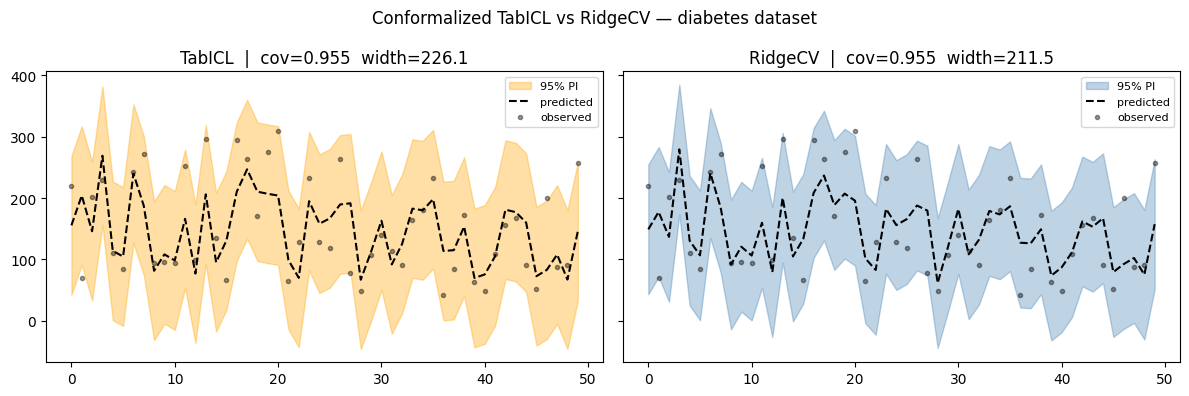
plt.suptitle("Conformalized TabICL vs RidgeCV — diabetes dataset")
plt.tight_layout()
plt.show()

Checkpoint 'tabicl-regressor-v2-20260212.ckpt' not cached.
 Downloading from Hugging Face Hub (jingang/TabICL).




tabicl-regressor-v2-20260212.ckpt:   0%|          | 0.00/114M (00:00, ?B/s)


TabICL      time=21.8s
TabICL      RMSE=54.4  coverage=0.955  avg_width=226.1
RidgeCV     time=0.0s
RidgeCV     RMSE=53.9  coverage=0.955  avg_width=211.5

 %load_ext rpy2.ipython # in a Colab notebook, use this

%R install.packages("reticulate")

%%R  # in Colab/Jupyter with rpy2; remove this line for pure R

library(reticulate)

# pip install tabicl nnetsauce scikit-learn matplotlib numpy

sklearn_ds  <- import("sklearn.datasets")
sklearn_ms  <- import("sklearn.model_selection")
sklearn_m   <- import("sklearn.metrics")
sklearn_lm  <- import("sklearn.linear_model")
tabicl      <- import("tabicl")
ns          <- import("nnetsauce")
np          <- import("numpy")
plt         <- import("matplotlib.pyplot")

# ── data ───────────────────────────────────────────────────
d       <- sklearn_ds$load_diabetes(return_X_y = TRUE)
X <- d((1)); y <- d((2))
sp      <- sklearn_ms$train_test_split(X, y,
             test_size = 0.2, random_state = 42L)
X_train <- sp((1)); X_test <- sp((2))
y_train <- sp((3)); y_test <- sp((4))

# ── helper: fit + evaluate ─────────────────────────────────
eval_model <- function(reg, name) {
  conf <- ns$PredictionInterval(reg, level = 95L)
  conf$fit(X_train, y_train)
  pi   <- conf$predict(X_test, return_pi = TRUE)

  cov  <- np$mean((pi$lower <= y_test) * (pi$upper >= y_test))
  wid  <- np$mean(pi$upper - pi$lower)
  rmse <- sqrt(sklearn_m$mean_squared_error(y_test, pi$mean))

  cat(sprintf("%-10s  RMSE=%.1f  coverage=%.3f  avg_width=%.1fn",
              name, rmse, cov, wid))
  invisible(pi)
}

# ── run both models ────────────────────────────────────────
pi_tabicl  <- eval_model(tabicl$TabICLRegressor(),  "TabICL")
pi_ridge   <- eval_model(sklearn_lm$RidgeCV(),       "RidgeCV")

# ── plot ───────────────────────────────────────────────────
max_idx <- 50L
x_range <- np$array(0:(max_idx - 1))

plot_pi <- function(pi, title, col) {
  x_fill <- np$concatenate(list(x_range, x_range(max_idx:1)))
  y_fill <- np$concatenate(list(
    pi$upper(1:max_idx), pi$lower(max_idx:1)))
  plt$fill(x_fill, y_fill, alpha=0.35, fc=col, ec="None", label="95% PI")
  plt$plot(x_range, pi$mean(1:max_idx), "k--", lw=1.5, label="predicted")
  plt$plot(x_range, y_test(1:max_idx), "k.", ms=6L, alpha=0.4, label="observed")
  plt$title(title); plt$legend(fontsize=8L)
}

fig <- plt$figure(figsize=c(12, 4))
plt$subplot(1L, 2L, 1L); plot_pi(pi_tabicl, "Conformalized TabICL", "orange")
plt$subplot(1L, 2L, 2L); plot_pi(pi_ridge,  "Conformalized RidgeCV", "steelblue")
plt$suptitle("Conformalized TabICL vs RidgeCV — diabetes dataset")
plt$tight_layout()
plt$show()

    WARNING: The R package "reticulate" only fixed recently
    an issue that caused a segfault when used with rpy2:
    https://github.com/rstudio/reticulate/pull/1188
    Make sure that you use a version of that package that includes
    the fix.
    TabICL      RMSE=54.4  coverage=0.955  avg_width=226.1
RidgeCV     RMSE=53.9  coverage=0.955  avg_width=211.5

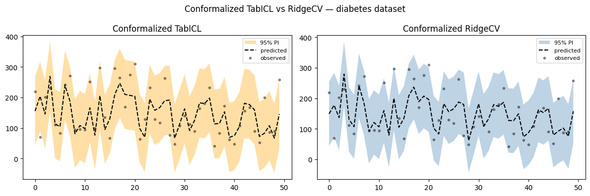
Probabil un set de date și asta uşor pentru un transformator. Conformalizarea modelelor simple îi ajută, în general, să obțină rate de acoperire apropiate de nivelul nominal, așa cum vedem pentru RidgeCV aici.