
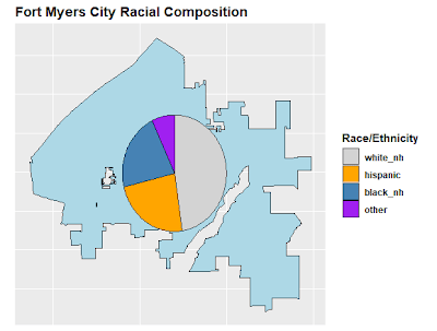
| Rasa (NH = non-hispanic) | Procent |
|---|---|
| Alb (NH) | 47,51% |
| hispanic (orice rasă) | 23,61% |
| Negru (NH) | 21,87% |
| Altele (NH) | 7,01% |
Suprapunerea tabelului de mai sus sub formă de diagramă circulară pe harta Fort Myers City dă următoarele:
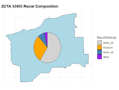
Apoi, am colectat datele și am desenat diagrama circulară pentru un singur ZCTA, 33905. Acest ZCTA are un procent mai mare de hispanici decât Fort Myers City și un procent mai mic de negri.

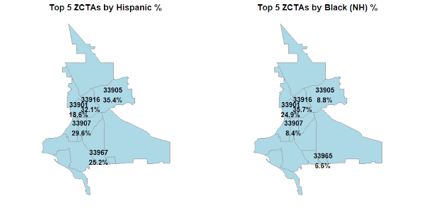
Am încercat inițial să creez o singură hartă cu o diagramă circulară separată pentru fiecare ZCTA, dar acea hartă era prea ocupată, deoarece multe ZCTA erau prea aproape unele de altele. Am decis că ceea ce îmi pasă cu adevărat era ZCTA cu cel mai mare procent de hispanici și ZCTA cu cel mai mare procent de negri:
Care este valoarea în toate acestea?
Care este valoarea în toate acestea? Farmacia, magazinul universal și serviciul de streaming video folosesc toate informațiile despre dvs. pentru a oferi recomandări personalizate bazate pe ceea ce cred că veți cumpăra sau veți urmări în continuare. Partidele noastre politice produc mesaje politice personalizate pentru diferite cartiere, pe baza a ceea ce consideră că sunt problemele politice majore ale rezidenților lor? Este rasa/etnia o variabilă importantă (deși, desigur, nu singura) în problemele politice ale oamenilor? Cred că poate partidele noastre politice ar trebui să se gândească să folosească mai mult informațiile demografice și geografice atunci când decid cum să comunice cu alegătorii.
cod R
Există o mulțime de coduri R. Am fost ajutat considerabil de Microsoft Copilot și Google Gemini.
# Race by ZCTA
# MY_KEY <- "xxxxx"
# Sys.setenv(CENSUS_API_KEY = "MY_KEY")

library(tidycensus)
library(tigris)
library(dplyr)
library(tidyr)
library(stringr)
library(sf)
library(ggplot2)
library(scatterpie)
library(gridExtra)

options(tigris_use_cache = TRUE)

# ------------------------------------------------------------
# Variable Definitions
# ------------------------------------------------------------

# 2020 Census P2 (Place-Level)
vars_p2 <- c(
  total     = "P2_001N",
  hispanic  = "P2_002N",
  white_nh  = "P2_005N",
  black_nh  = "P2_006N",
  aian_nh   = "P2_007N",
  asian_nh  = "P2_008N",
  nhpi_nh   = "P2_009N",
  other_nh  = "P2_010N",
  multi_nh  = "P2_011N"
)

# 2020 Census DHC ZCTA Variables
vars_p5 <- c(
  total_pop = "P5_001N",
  white_nh  = "P5_003N",
  black_nh  = "P5_004N",
  aian_nh   = "P5_005N",
  asian_nh  = "P5_006N",
  nhpi_nh   = "P5_007N",
  other_nh  = "P5_008N",
  multi_nh  = "P5_009N",
  hispanic  = "P5_010N"
)

# ACS Variables (for individual ZCTA analysis)
vars_acs <- c(
  total     = "B03002_001",
  white_nh  = "B03002_003",
  black_nh  = "B03002_004",
  aian_nh   = "B03002_005",
  asian_nh  = "B03002_006",
  nhpi_nh   = "B03002_007",
  other_nh  = "B03002_008",
  multi_nh  = "B03002_009",
  hispanic  = "B03002_012"
)

# ------------------------------------------------------------
# Geography
# ------------------------------------------------------------

places_fl <- places(state = "FL", year = 2020)

fort_myers_shape <- places_fl %>%
  filter(NAME == "Fort Myers")

zctas_fl <- zctas(
  year = 2020,
  cb = TRUE,
  starts_with = "339"
)

# ------------------------------------------------------------
# CITY OF FORT MYERS RACE TABLE
# ------------------------------------------------------------

race_eth_city <- get_decennial(
  geography = "place",
  state = "FL",
  variables = vars_p2,
  year = 2020,
  sumfile = "pl",
  output = "wide"
) %>%
  filter(NAME == "Fort Myers city, Florida")

race_city <- race_eth_city %>%
  transmute(
    white_nh,
    hispanic,
    black_nh,
    other =
      aian_nh +
      asian_nh +
      nhpi_nh +
      other_nh +
      multi_nh
  )

race_table_city <- race_city %>%
  pivot_longer(
    everything(),
    names_to = "race",
    values_to = "population"
  ) %>%
  mutate(
    pct = population / sum(population)
  )

print(race_table_city)

# ------------------------------------------------------------
# CITY OF FORT MYERS MAP
# ------------------------------------------------------------

ggplot(fort_myers_shape) +
  geom_sf(
    fill = "lightblue",
    color = "black"
  ) +
  labs(
    title = "City of Fort Myers (2020 Census Boundary)"
  ) +
  theme_minimal() +
  theme(
    plot.title = element_text(face = "bold"),
    axis.text  = element_blank(),
    axis.ticks = element_blank()
  )

# ------------------------------------------------------------
# CITY PIE CHART MAP
# ------------------------------------------------------------

ctr <- st_coordinates(
  st_centroid(
    st_union(fort_myers_shape)
  )
)

pie_df_city <- cbind(
  data.frame(
    x = ctr(1),
    y = ctr(2)
  ),
  race_city
)

ggplot() +
  geom_sf(
    data = fort_myers_shape,
    fill = "lightblue",
    color = "black"
  ) +
  geom_scatterpie(
    data = pie_df_city,
    aes(x = x, y = y, r = 0.03),
    cols = names(race_city)
  ) +
  scale_fill_manual(
    values = c(
      white_nh = "lightgray",
      hispanic = "orange",
      black_nh = "steelblue",
      other = "purple"
    )
  ) +
  labs(
    title = "Fort Myers City Racial Composition",
    fill = "Race/Ethnicity"
  ) +
  coord_sf() +
  theme(
    plot.title = element_text(face = "bold"),
    axis.title = element_blank(),
    axis.text = element_blank(),
    axis.ticks = element_blank(),
    legend.title = element_text(face = "bold"),
    legend.text = element_text(face = "bold")
  )

# ------------------------------------------------------------
# GREATER FORT MYERS ZCTA MAP
# ------------------------------------------------------------

fort_myers_zctas <- zctas_fl %>%
  st_filter(fort_myers_shape,
            .predicate = st_intersects)

ggplot() +
  geom_sf(
    data = fort_myers_zctas,
    fill = "lightblue",
    color = "black",
    alpha = 0.6
  ) +
  geom_sf(
    data = fort_myers_shape,
    fill = NA,
    color = "red",
    linewidth = 1.8,
    linetype = "dashed"
  ) +
  geom_sf_label(
    data = fort_myers_zctas,
    aes(label = ZCTA5CE20),
    size = 3,
    fontface = "bold"
  ) +
  labs(
    title = "Greater Fort Myers Area by ZCTA",
    subtitle = "Dashed red line indicates city limits",
    x = "",
    y = "") +
  theme_minimal() +
  theme(
    plot.title = element_text(face = "bold"),
    plot.subtitle = element_text(face = "bold"),
    axis.text = element_blank(),
    axis.ticks = element_blank()
  )

# ------------------------------------------------------------
# SINGLE ZCTA ANALYSIS (33905)
# ------------------------------------------------------------

race_eth_33905 <- get_acs(
  geography = "zcta",
  variables = vars_acs,
  year = 2020,
  output = "wide"
) %>%
  filter(GEOID == "33905")

race_33905 <- race_eth_33905 %>%
  transmute(
    white_nh = white_nhE,
    hispanic = hispanicE,
    black_nh = black_nhE,
    other =
      aian_nhE +
      asian_nhE +
      nhpi_nhE +
      other_nhE +
      multi_nhE
  )

race_table_33905 <- race_33905 %>%
  pivot_longer(
    everything(),
    names_to = "race",
    values_to = "population"
  ) %>%
  mutate(
    pct = population / sum(population)
  )

print(race_table_33905)

# ------------------------------------------------------------
# ZCTA 33905 PIE MAP
# ------------------------------------------------------------

zcta_33905 <- zctas_fl %>%
  filter(ZCTA5CE20 == "33905")

coords_33905 <- st_coordinates(
  st_centroid(zcta_33905)
)

pie_df_33905 <- race_33905 %>%
  mutate(
    x = coords_33905(1,1),
    y = coords_33905(1,2)
  )


ggplot() +
  geom_sf(
    data = zcta_33905,
    fill = "lightblue",
    color = "black"
  ) +
  geom_scatterpie(
    data = pie_df_33905,
    aes(x = x, y = y, r = 0.025),
    cols = c(
      "white_nh",
      "hispanic",
      "black_nh",
      "other"
    )
  ) +
  scale_fill_manual(
    values = c(
      white_nh = "lightgray",
      hispanic = "orange",
      black_nh = "steelblue",
      other = "purple"
    )
  ) +
  labs(
    title = "ZCTA 33905 Racial Composition",
    fill = "Race/Ethnicity"
  ) +
  coord_sf() +
  theme_minimal() +
  theme(
    plot.title = element_text(face = "bold"),
    axis.title = element_blank(),
    axis.text = element_blank(),
    axis.ticks = element_blank()
  )

# ------------------------------------------------------------
# ALL FORT MYERS AREA ZCTAS
# ------------------------------------------------------------

fort_myers_list <- c(
  "33901","33903","33905","33907",
  "33908","33912","33913","33916",
  "33917","33919","33931","33965",
  "33966","33967"
)

fort_myers_master <- get_decennial(
  geography = "zcta",
  variables = vars_p5,
  year = 2020,
  sumfile = "dhc",
  output = "wide",
  geometry = TRUE
)

fort_myers_projected <- fort_myers_master %>%
  filter(GEOID %in% fort_myers_list) %>%
  mutate(
    zcta = str_extract(NAME, "\d{5}"),
    pct_hispanic =
      100 * hispanic / total_pop,
    pct_black_nh =
      100 * black_nh / total_pop,
    minority_other_nh =
      aian_nh +
      asian_nh +
      nhpi_nh +
      other_nh +
      multi_nh
  ) %>%
  st_transform(2237)

# ------------------------------------------------------------
# POPULATION MATRIX
# ------------------------------------------------------------

fort_myers_population_table <- fort_myers_projected %>%
  st_drop_geometry() %>%
  select(
    zcta,
    total_pop,
    white_nh,
    hispanic,
    black_nh,
    minority_other_nh
  ) %>%
  arrange(zcta)

print(fort_myers_population_table)

# ------------------------------------------------------------
# CENTROIDS
# ------------------------------------------------------------

centroids_master <- fort_myers_projected %>%
  st_centroid() %>%
  mutate(
    X = st_coordinates(.)(,1),
    Y = st_coordinates(.)(,2)
  ) %>%
  st_drop_geometry()

top_5_hispanic <- centroids_master %>%
  slice_max(
    pct_hispanic,
    n = 5
  ) %>%
  mutate(
    label_text =
      paste0(
        zcta,
        "n",
        round(pct_hispanic, 1),
        "%"
      )
  )

top_5_black <- centroids_master %>%
  slice_max(
    pct_black_nh,
    n = 5
  ) %>%
  mutate(
    label_text =
      paste0(
        zcta,
        "n",
        round(pct_black_nh, 1),
        "%"
      )
  )

# ------------------------------------------------------------
# BASE MAP
# ------------------------------------------------------------

base_map <- ggplot() +
  geom_sf(
    data = fort_myers_projected,
    fill = "lightblue",
    color = "gray60"
  ) +
  theme_minimal() +
  theme(
    plot.title = element_text(
      face = "bold",
      hjust = .5
    ),
    axis.title = element_blank(),
    axis.text = element_blank(),
    panel.grid = element_blank()
  ) +
  coord_sf(datum = NA)

# ------------------------------------------------------------
# TOP 5 HISPANIC
# ------------------------------------------------------------

map_hispanic <- base_map +
  geom_text(
    data = top_5_hispanic,
    aes(
      X,
      Y,
      label = label_text
    ),
    fontface = "bold"
  ) +
  labs(
    title = "Top 5 ZCTAs by Hispanic %"
  )

# ------------------------------------------------------------
# TOP 5 BLACK NH
# ------------------------------------------------------------

map_black <- base_map +
  geom_text(
    data = top_5_black,
    aes(
      X,
      Y,
      label = label_text
    ),
    fontface = "bold"
  ) +
  labs(
    title = "Top 5 ZCTAs by Black (NH) %"
  )

# ------------------------------------------------------------
# DISPLAY FINAL MAPS
# ------------------------------------------------------------

grid.arrange(
  map_hispanic,
  map_black,
  ncol = 2
)
Sfârşit
