(Acest articol a fost publicat pentru prima dată pe https://pacha.dev/blogși cu amabilitate a contribuit la R-bloggeri). (Puteți raporta problema legată de conținutul acestei pagini aici)
Doriți să vă distribuiți conținutul pe R-bloggeri? dați clic aici dacă aveți un blog, sau aici dacă nu aveți.
Scopul corelațiilor false este de a menține în viață exemplele uimitoare de la Tyler Vigen. Din păcate, începând cu 2023-10-09, site-ul web este oprit, așa cum au observat studenții mei. Prin urmare, am decis să folosesc instantaneul de la Internet Wayback Machine pentru a salva seturile de date din 2023-06-07.
Instalare
Puteți instala versiunea CRAN a corelațiilor false cu:
install.packages("spuriouscorrelations")
Puteți instala versiunea de dezvoltare a spuriouscorelations cu:
remotes::install_github("pachadotdev/spuriouscorrelations")
Exemplu
Pachetul acoperă mai multe exemple pentru diferite corelații false (și curioase).
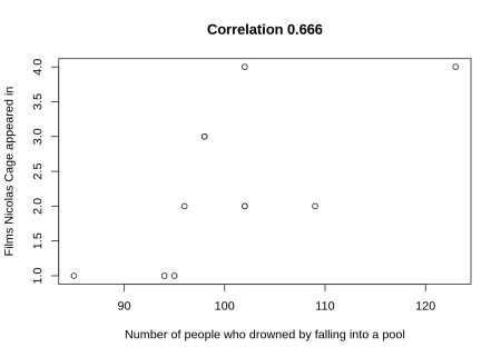
Iată un exemplu de bază care vă arată cum să reprezentați o corelație falsă pentru variabile
- x: Numărul de persoane care s-au înecat căzând într-o piscină
- y: Filmele în care a apărut Nicolas Cage
library(spuriouscorrelations)
library(tinyplot)

pool_drownings
   year   x y
1  1999 109 2
2  2000 102 2
3  2001 102 2
4  2002  98 3
5  2003  85 1
6  2004  95 1
7  2005  96 2
8  2006  98 3
9  2007 123 4
10 2008  94 1
11 2009 102 4
cor(pool_drownings$x, pool_drownings$y)
(1) 0.6660043
tinyplot(
  y ~ x,
  data = pool_drownings,
  main = sprintf("Correlation %s", round(cor(pool_drownings$x, pool_drownings$y), 3)),
  xlab = "Number of people who drowned by falling into a pool",
  ylab = "Films Nicolas Cage appeared in"
)
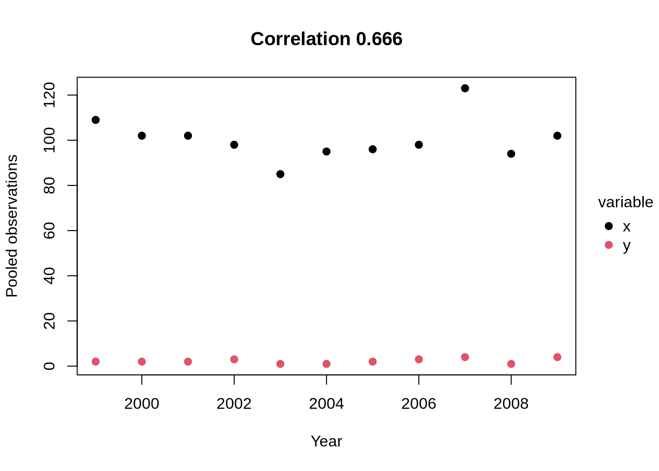
Convertirea datelor în format lung simplifică reprezentarea grafică a ambelor variabile pe an:
pool_drownings_2 <- reshape(
  pool_drownings,
  varying = c("x", "y"),  # columns to collapse
  v.names = "value",      # name of the new value column
  timevar = "variable",   # name of the new ID column
  times = c("x", "y"),    # values to populate the ID column
  direction = "long"      # target format
)

pool_drownings_2
     year variable value id
1.x  1999        x   109  1
2.x  2000        x   102  2
3.x  2001        x   102  3
4.x  2002        x    98  4
5.x  2003        x    85  5
6.x  2004        x    95  6
7.x  2005        x    96  7
8.x  2006        x    98  8
9.x  2007        x   123  9
10.x 2008        x    94 10
11.x 2009        x   102 11
1.y  1999        y     2  1
2.y  2000        y     2  2
3.y  2001        y     2  3
4.y  2002        y     3  4
5.y  2003        y     1  5
6.y  2004        y     1  6
7.y  2005        y     2  7
8.y  2006        y     3  8
9.y  2007        y     4  9
10.y 2008        y     1 10
11.y 2009        y     4 11
tinyplot(
  value ~ year | variable, # "|" indicates the groping variable for the legend
  data = pool_drownings_2,
  main = sprintf("Correlation %s", round(cor(pool_drownings$x, pool_drownings$y), 3)),
  xlab = "Year",
  ylab = "Pooled observations",
  pch = 19 # solid dot shape
)

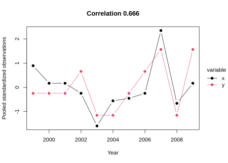
Ce zici de standardizarea variabilelor pentru a evita problema de vizibilitate la scară diferită?
pool_drownings_3 <- pool_drownings

pool_drownings_3$x <- (pool_drownings_3$x - mean(pool_drownings_3$x)) / sd(pool_drownings_3$x)
pool_drownings_3$y <- (pool_drownings_3$y - mean(pool_drownings_3$y)) / sd(pool_drownings_3$y)

pool_drownings_3 <- reshape(
  pool_drownings_3,
  varying = c("x", "y"),  # columns to collapse
  v.names = "value",      # name of the new value column
  timevar = "variable",   # name of the new ID column
  times = c("x", "y"),    # values to populate the ID column
  direction = "long"      # target format
)

pool_drownings_3
     year variable      value id
1.x  1999        x  0.8952867  1
2.x  2000        x  0.1696333  2
3.x  2001        x  0.1696333  3
4.x  2002        x -0.2450258  4
5.x  2003        x -1.5926679  5
6.x  2004        x -0.5560201  6
7.x  2005        x -0.4523554  7
8.x  2006        x -0.2450258  8
9.x  2007        x  2.3465935  9
10.x 2008        x -0.6596849 10
11.x 2009        x  0.1696333 11
1.y  1999        y -0.2470999  1
2.y  2000        y -0.2470999  2
3.y  2001        y -0.2470999  3
4.y  2002        y  0.6589330  4
5.y  2003        y -1.1531327  5
6.y  2004        y -1.1531327  6
7.y  2005        y -0.2470999  7
8.y  2006        y  0.6589330  8
9.y  2007        y  1.5649658  9
10.y 2008        y -1.1531327 10
11.y 2009        y  1.5649658 11
tinyplot(
  value ~ year | variable, # "|" indicates the groping variable for the legend
  data = pool_drownings_3,
  main = sprintf("Correlation %s", round(cor(pool_drownings$x, pool_drownings$y), 3)),
  xlab = "Year",
  ylab = "Pooled standardized observations",
  pch = 19, # solid dot shape
  type = "b" # add line to see the trend clearly
)