Date climatice SIM2 | R-bloggeri

(Acest articol a fost publicat pentru prima dată pe r.iresmi.netși cu amabilitate a contribuit la R-bloggeri). (Puteți raporta problema legată de conținutul acestei pagini aici)

Doriți să vă distribuiți conținutul pe R-bloggeri? dați clic aici dacă aveți un blog, sau aici dacă nu aveți.

O diagramă a anomaliilor de temperatură în Franța sub formă de dungi albastre și roșii — Schimbarea temperaturii în Franța – CC-BY de Universitatea din Reading

Pe măsură ce Franța intră în al doilea val de căldură din 2026, putem produce diagrame mai detaliate decât vizualizările excelente oferite de ShowYourStripes?

MétéoFrance oferă setul său lunar de date SIM2, deși pe o perioadă mai scurtă de timp (în prezent 1970–2025). Setul de date include temperatura, precipitațiile și alte variabile pe o grilă cu rezoluție de 8 km.

Vom selecta un oraș francez, vom prelua coordonatele geografice ale acestuia, vom construi grila pentru o anumită lună în perioada 1970-2025, vom extrage datele din grila din acea locație și vom reprezenta grafic anomalia de temperatură.

Vom folosi {terra} pentru a crea grila din fișierele tabulare care conțin centre de celule și variabile meteorologice și terra::extract() pentru a obține toate temperaturile.

library(tidyverse)
library(fs)
library(janitor)
library(osmdata)
library(sf)
library(terra)
library(glue)
library(memoise)

invisible(
  Sys.setlocale(category = "LC_ALL", 
                locale = "en_GB.UTF8"))


#' Geolocate using OSM (Nominatim API)
#'
#' using first result
#' Memoized function
#'
#' @param location (char): place name (geocodable via OSM)
#'
#' @returns (SpatVector): first result
geolocate <- memoise(function(location) {
  loc <- getbb(location, format_out = "sf_polygon")  |> 
    st_point_on_surface() |>
    slice_head(n = 1)
  
  message(glue("{loc$display_name} — WGS84 : {loc$geometry}"))
  
  return(loc|>
           st_transform("IGNF:NTFLAMB2E") |>
           as("SpatVector"))
})

#' Generate a monthly temperature chart since 1970
#'
#' @param sim2 (data.frame): Météo-France SIM2 data over the period
#' @param month (char): month number "01"..."12"
#' @param location (char): place name (geocodable via OSM); memoized
#' @param output_dir (char): directory path where a PNG file will be written, if not NULL
#'
#' @returns (ggplot and optionally a file on disk)
generate_chart <- function(
    sim2,
    month,
    location,
    output_dir = NULL) {
  stopifnot(month %in% sprintf("%02d", 1:12))
  month_name <- format(ymd(glue("0000-{month}-01")), "%B")
  
  sim2_raster <- sim2 |>
    filter(str_detect(date, glue("{month}$"))) |>
    mutate(
      x = lambx * 100,
      y = lamby * 100,
      layer = date,
      temp = t,
      .keep = "none") |>
    rast(
      type = "xylz",
      crs = "IGNF:NTFLAMB2E")
  
  loc <- geolocate(location)
  
  temperatures <- sim2_raster |>
    terra::extract(loc) |>
    select(-ID) |>
    pivot_longer(
      cols = everything(),
      names_to = "month",
      values_to = "temperature") |>
    mutate(
      year = as.integer(str_sub(month, 1, 4)),
      anomaly = temperature - mean(temperature(year >= 1991 & year <= 2020),
                                   na.rm = TRUE))
  
  p <- temperatures |>
    ggplot(aes(year, anomaly)) +
    geom_col(aes(fill = anomaly)) +
    geom_smooth(method = "loess",
                formula = y ~ x) +
    scale_fill_gradient2(
      high = scales::muted("red"),
      mid = "white",
      low = scales::muted("blue")) +
    scale_x_continuous(breaks = scales::breaks_pretty()) +
    scale_y_continuous(breaks = scales::breaks_pretty()) +
    labs(
      title = glue("Average monthly anomaly temperature — {month_name}"),
      subtitle = location,
      x = "year",
      y = "departure from average* (°C)",
      fill = "°C",
      caption = glue(
        "https://r.iresmi.net/ — {Sys.Date()}
         data: Météo-France SIM2 — *baseline: 1991–2020 normal for {month_name}")) +
    theme(
      text = element_text(family = "Ubuntu"),
      plot.caption = element_text(size = 7))
  
  if (!is.null(output_dir)) {
    dir_create(output_dir)
    
    ggsave(
      glue("{output_dir}/tm_{month}_{make_clean_names(location)}.png"),
      plot = p,
      width = 20,
      height = 20 / 1.618,
      units = "cm",
      dpi = 150)
  }
  
  return(p)
}

Datele sunt o grămadă de CSV comprimate.

# https://meteo.data.gouv.fr/datasets/65e040c50a5c6872ebebc711
# Climate change data - monthly SIM
# all files MENS_SIM2_*-*.csv.gz
sim2 <- dir_ls("data") |>
  read_delim(
    delim = ";",
    locale = locale(decimal_mark = "."),
    name_repair = make_clean_names)

Acum numim doar funcția noastră.

generate_chart(sim2,
               month = "06",
               location = "Paris, France")

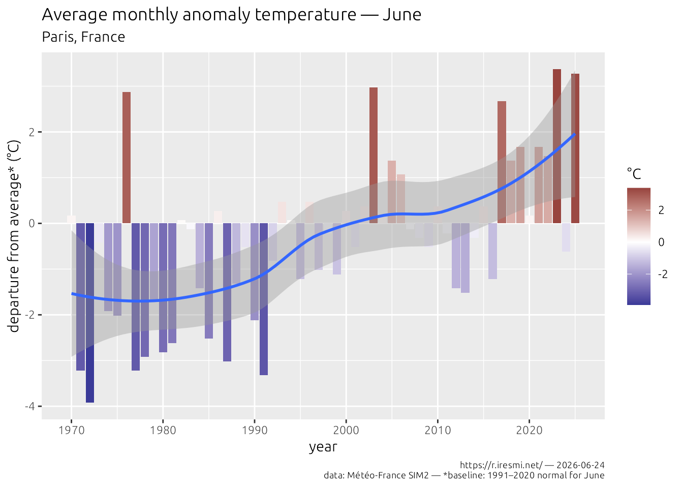
Graficul de bare a anomaliei de temperatură la Paris — Figura 1: Temperatura din iunie la Paris 1970–2025

Dacă vrem în fiecare lună:

# for each month
sprintf("%02d", 1:12) |>
  map((x) generate_chart(sim2,
                           month = x,
                           location = "Grenoble, France",
                           output_dir = "results"), 
  .progress = TRUE)

Rețineți că scările nu sunt constante pe diagrame; dacă vrem să comparăm luna (sau locurile) ar trebui să fixăm axa y și scala de culori. Este lăsat ca un exercițiu cititorului dacă doriți să faceți un poster frumos…

Date climatice SIM2 | R-bloggeri

LĂSAȚI UN MESAJ Renunțați la răspuns